Chapter 7: Complex Number Calculus

Terms:
Cauchy-Riemann equations
contour integration 
holomorphic functions 

Consider the function \(f(x)\) where \(z\) is a complex number. The definite integral on complex variable \(z\): \[\int_{a}^{b}f(z)dz = g(b) - g(a)\] \(\bullet\) there are multiple paths from \(a\) to \(b\) when we are on a complex plane
\(\bullet\) the answer would be the same along all such paths which can be obtained via continuous deformation of the original
\(\star\) results from "fundamental theorem of exterior calculus"


If a function has an undefined value, then this yields a hole on the complex plane which means that there may exist multiple integration paths which cannot be related via continuous deformation.
\(\bullet\) these continuous deformations are called "homologous deformations"
\(\bullet\) paths related by homologous deformations are in the same "homology class"
\(\bullet\) homologous deformations can have orientations that cancel when a path loops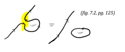

Consider \(f(z) = \frac{1}{z}\) with a complex variable. The definite integral is given by \[\int_{a}^{b}\frac{dz}{z} = \log{b} - \log{a}\] where \(a\) and \(b \in \mathbb{C}\). Recall that the logarithm of a complex value can be expressed as the logarithm of a real value and \(i\theta\). That is, we can express \[\log{b} = \log{r} + i\theta\] \[\log{a} = \log{s} + i\phi\] Varying only one of the complex numbers above, we can see that we can increase the phase (\(\theta\)) of the integral by \(2\pi\) with each positive rotation about the origin of the path of integration.

Closed Contours

As described above, one can visualize closed contour integration graphically by:
\(\bullet\) varying the 2nd path first
\(\bullet\) then varying the first path in the reverse direction (since it is being subtracted)
\(\bullet\) cancelling out alternate orientation portions
The loop/closed path to the right below is called a contour

\(\star\) the contour is independent of the location of \(a\) and \(b\)
This gives us the notion of a closed contour integral \[\oint \frac{dz}{z} = 2\pi i\] For a holomorphic function \(f(z)\), its value at the origin is given by the Cauchy formula as \[\frac{1}{2\pi i} \oint \frac{f(z)}{z}dz = f(0)\] the left is essentially any loop around the origin
\(\bullet\) the nth derivative \(f^{n}(0)\) can be obtained from \[\frac{n!}{2\pi i}\oint\frac{f(z)(z^{n+1}}dz = f^{n}(0)\]
\(\bullet\) more generally, about any point \(p\) we have \[\frac{1}{2\pi i}\oint\frac{f(z)}{z-p}dz = f(p)\] \[\frac{n!}{2\pi i}\oint\frac{f(z)}{(z-p)^{n+1}}dz=f^{n}(p)\] "Complex smoothness implies analytcity (holomorphicity) at every point of the domain." (pg. 128)

Using these variations of Cauchy formulas, we can write a power series about any point in an open, complex-smooth region. Further, this power series will be convergent.
\(\bullet\) singular point = singularity of \(f(z)\) for \(z\) complex
\(\bullet\) regular point = point at which \(f(z)\) does not have a singularity/ where it is holomorphic
Singular and regular points are covered at the start of the Differential Topology text.