|
The necessity for knot invariants arises from the need for a mathematically precise way to characterize and compare knots - ie. to determine if 2 knots are the same knot or if a given knot is nontrivial (not really a knot/the unknot) and likewise for links.
The first such invariant I was introduced to is the Jones Polynomial which is constructed from the bracket polynomial which is defined in terms of the conditions:
1. \(\langle L \rangle = a\langle L_{A} \rangle + b\langle L_{B} \rangle\)
2. \(\langle L \sqcup \bigcirc \rangle = c \langle L \rangle\) 3. \(\langle \bigcirc \rangle = 1\)
For a given polynomial, relations between the variables a, b, and c are determined such than the resulting polynomial is invariant under each of the 3 Reidemeister moves.
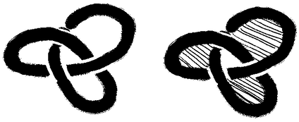
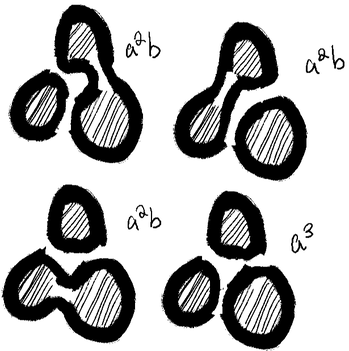
The most straight forward and (brute forced) method to compute the bracket polynomial for a knot with n crossings is by identifying alternating regions created by the knot as regions A and B like so:
The generalized formula for the bracket polynomial is then
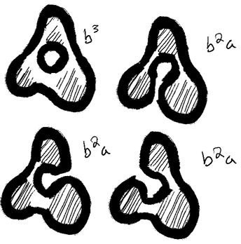
\[\langle L \rangle = \sum_{s}a^{\alpha(s)}b^{\beta(s)}c^{\gamma(s)-1} = \sum_{s}a^{\alpha(s)-\beta(s)}(-a^{2}-a^{-2})^{\gamma(s)-1}\] where \(s\) is the identifier of each of the \(2^{n}\) states and \(\alpha(s)\) is the exponent on \(a\), \(\beta(s)\) is the exponent on \(b\) and \(\gamma(s)\) is the number of circles created.
For the example above, we get \begin{split} \langle L \rangle & = a^{3}(-a^{2}-a^{-2})^{2} + (a^{-3} + 3a)(-a^{2}-a^{-2}) + 3a^{-1}\\ & = a^{7} - a^{3} - a^{-5} \end{split}
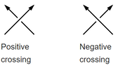
For oriented knots and links we can then define the writhe number as
\[w(L) = \sum_{i}\epsilon_{i}\] where \(i\) is the sum over the \(n\) crossings and \(\epsilon\) is defined as + or -1 as per the diagram below
We can now define the Kauffman polynomial as
\[X(L) = (-a)^{-3w(L)}\langle |L| \rangle\]
By virtue of it's construction, the Kauffman polynomial is invariant under each of the Reidemeister moves and thus constitutes a an isotopy invariant for oriented knots and links. The Jones polynomial is then very easily obtained from the Kauffman polynomial by applying the map
\[a \mapsto q^{-\frac{1}{4}}\]
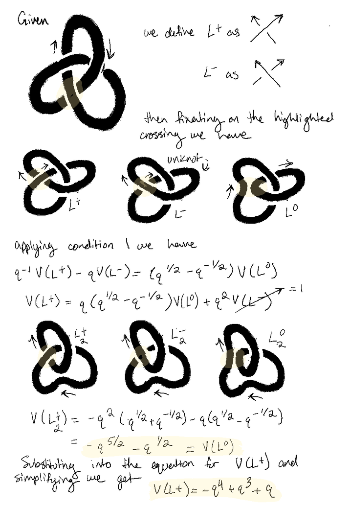
The Jones polynomial satisfies the relations 1. \(q^{-1}V(L^{+}) - qV(L^{-}) = (q^{\frac{1}{2}} - q^{-\frac{1}{2}})V(L^{o})\) ...note, this is the skein relation 2. \(V(L \sqcup \bigcirc) = -(q^{-\frac{1}{2}} + q^{\frac{1}{2}})V(L)\) 3. \(V(\bigcirc) = 1\)
An easier way to calculate the Jones polynomial however is to define the positive and negative links as per the relations shown above and apply the algorithm shown below for the trefoil knot.
The Jones polynomial can tell us if two knots are different or nonisotopic if they have two different Jones polynomials. However, it is important to note that the Jones polynomial cannot guarantee that two knots with the same Jones polynomial are isotopic or the same. The Jones polynomial can also be defined in terms of 2 variables as
\[\frac{1}{\sqrt{\lambda}\sqrt{q}}\chi(L^{+}) - \sqrt{\lambda}\sqrt{q}\chi(L^{-}) = \frac{\sqrt{q}-1}{\sqrt{q}}\chi(L^{o})\]
This version of the Jones polynomial can then be used to obtain any of these common invariants via a change of variables:
Conway polynomial: \(\mapsto \nabla(L^{+}) - \nabla(L^{-}) = z\nabla(L^{o})\)
Alexander polynomial: \(\mapsto \Delta(L^{+}) - \Delta(L^{-}) = \frac{1}{\sqrt{1 - t^{2}}}\Delta(L^{o}) \) HOMFLY polynomial: \(\mapsto x\mathcal{P}(L^{+}) - t\mathcal{P}(L^{-}) = \mathcal{P}(L^{o})\)
0 Comments
Leave a Reply. |
Archives
December 2021
Categories |
 RSS Feed